|
Open CASCADE Technology
7.0.0
|
|
|
Open CASCADE Technology
7.0.0
|
|
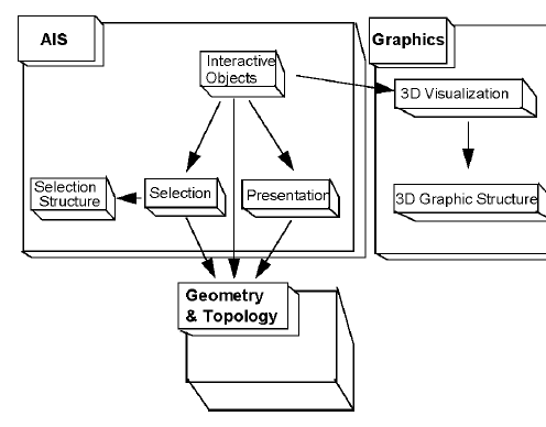
Visualization in Open CASCADE Technology is based on the separation of:
Presentations are managed through the Presentation component, and selection through the Selection component.
Application Interactive Services (AIS) provides the means to create links between an application GUI viewer and the packages, which are used to manage selection and presentation, which makes management of these functionalities in 3D more intuitive and consequently, more transparent.
AIS uses the notion of the interactive object, a displayable and selectable entity, which represents an element from the application data. As a result, in 3D, you, the user, have no need to be familiar with any functions underlying AIS unless you want to create your own interactive objects or selection filters.
If, however, you require types of interactive objects and filters other than those provided, you will need to know the mechanics of presentable and selectable objects, specifically how to implement their virtual functions. To do this requires familiarity with such fundamental concepts as the sensitive primitive and the presentable object.
The the following packages are used to display 3D objects:
The packages used to display 3D objects are also applicable for visualization of 2D objects.
The figure below presents a schematic overview of the relations between the key concepts and packages in visualization. Naturally, "Geometry & Topology" is just an example of application data that can be handled by AIS, and application-specific interactive objects can deal with any kind of data.
For advanced information on visualization algorithms, see our E-learning & Training offerings.
In Open CASCADE Technology, presentation services are separated from the data, which they represent, which is generated by applicative algorithms. This division allows you to modify a geometric or topological algorithm and its resulting objects without modifying the visualization services.
Displaying an object on the screen involves three kinds of entities:
The purpose of a presentable object is to provide the graphical representation of an object in the form of Graphic3d structure. On the first display request, it creates this structure by calling the appropriate algorithm and retaining this framework for further display.
Standard presentation algorithms are provided in the StdPrs and Prs3d packages. You can, however, write specific presentation algorithms of your own, provided that they create presentations made of structures from the Graphic3d packages. You can also create several presentations of a single presentable object: one for each visualization mode supported by your application.
Each object to be presented individually must be presentable or associated with a presentable object.
The viewer allows interactively manipulating views of the object. When you zoom, translate or rotate a view, the viewer operates on the graphic structure created by the presentable object and not on the data model of the application. Creating Graphic3d structures in your presentation algorithms allows you to use the 3D viewers provided in Open CASCADE Technology for 3D visualisation.
The interactive context controls the entire presentation process from a common high-level API. When the application requests the display of an object, the interactive context requests the graphic structure from the presentable object and sends it to the viewer for displaying.
Presentation involves at least the AIS, PrsMgr, StdPrs and V3d packages. Additional packages, such as Prs3d and Graphic3d may be used if you need to implement your own presentation algorithms.
The shape is created using the BRepPrimAPI_MakeWedge command. An AIS_Shape is then created from the shape. When calling the Display command, the interactive context calls the Compute method of the presentable object to calculate the presentation data and transfer it to the viewer. See figure below.

Standard OCCT selection algorithm is represented by 2 parts: dynamic and static. Dynamic selection causes objects to be automatically highlighted as the mouse cursor moves over them. Static selection allows to pick particular object (or objects) for further processing.
There are 3 different selection types:
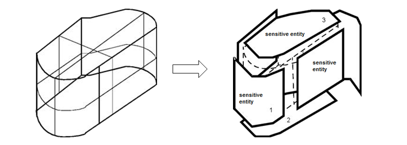
For OCCT selection algorithm, all selectable objects are represented as a set of sensitive zones, called sensitive entities. When the mouse cursor moves in the view, the sensitive entities of each object are analyzed for collision.
This section introduces basic terms and notions used throughout the algorithm description.
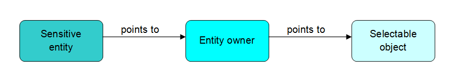
Sensitive entities in the same way as entity owners are links between objects and the selection mechanism.
The purpose of entities is to define what parts of the object will be selectable in particular. Thus, any object that is meant to be selectable must be split into sensitive entities (one or several). For instance, to apply face selection to an object it is necessary to explode it into faces and use them for creation of a sensitive entity set.
Entities are used as internal units of the selection algorithm and do not contain any topological data, hence they have a link to an upper-level interface that maintains topology-specific methods.
Each sensitive entity stores a reference to its owner, which is a class connecting the entity and the corresponding selectable object. Besides, owners can store any additional information, for example, the topological shape of the sensitive entity, highlight colors and methods, or if the entity is selected or not.
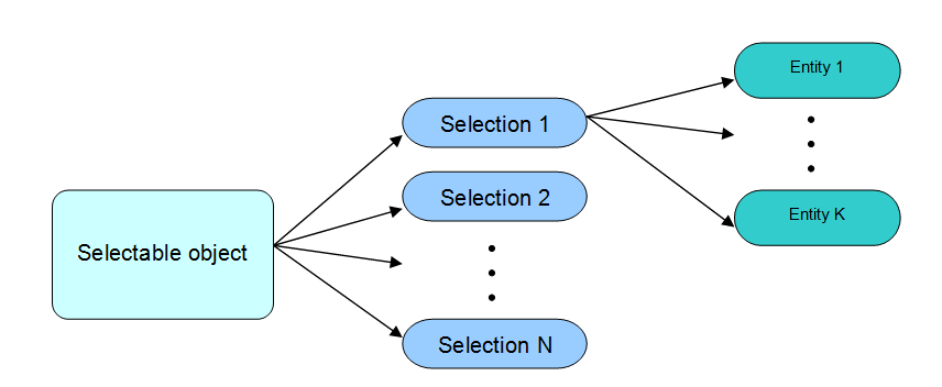
To simplify the handling of different selection modes of an object, sensitive entities linked to its owners are organized into sets, called selections.
Each selection contains entities created for a certain mode along with the sensitivity and update states.
Selectable object stores information about all created selection modes and sensitive entities.
All successors of a selectable object must implement the method that splits its presentation into sensitive entities according to the given mode. The computed entities are arranged in one selection and added to the list of all selections of this object. No selection will be removed from the list until the object is deleted permanently.
For all standard OCCT shapes, zero mode is supposed to select the whole object (but it may be redefined easily in the custom object). For example, the standard OCCT selection mechanism and AIS_Shape determine the following modes:
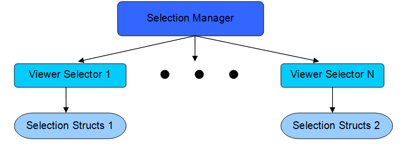
For each OCCT viewer there is a Viewer selector class instance. It provides a high-level API for the whole selection algorithm and encapsulates the processing of objects and sensitive entities for each mouse pick.
The viewer selector maintains activation and deactivation of selection modes, launches the algorithm, which detects candidate entities to be picked, and stores its results, as well as implements an interface for keeping selection structures up-to-date.
Selection manager is a high-level API to manipulate selection of all displayed objects. It handles all viewer selectors, activates and deactivates selection modes for the objects in all or particular selectors, manages computation and update of selections for each object. Moreover, it keeps selection structures updated taking into account applied changes.
All three types of OCCT selection are implemented as a single concept, based on the search for overlap between frustum and sensitive entity through 3-level BVH tree traversal.
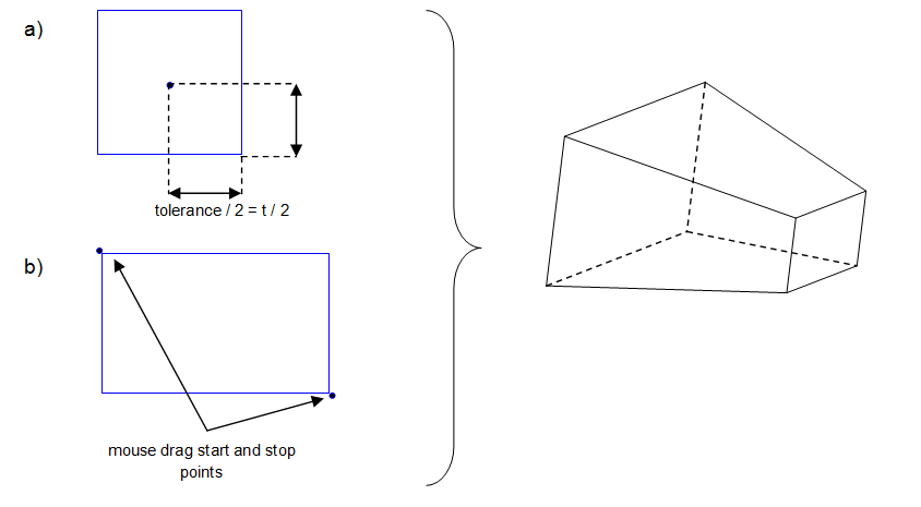
The first step of each run of selection algorithm is to build the selection frustum according to the currently activated selection type.
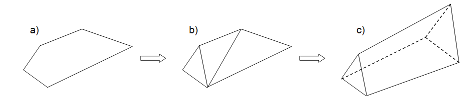
For the point or the rectangular selection the base of the frustum is a rectangle built in conformity with the pixel tolerance or the dimensions of a user-defined area, respectively. For the polyline selection, the polygon defined by the constructed line is triangulated and each triangle is used as the base for its own frustum. Thus, this type of selection uses a set of triangular frustums for overlap detection.
The frustum length is limited by near and far view volume planes and each plane is built parallel to the corresponding view volume plane.
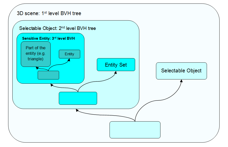
To maintain selection mechanism at the viewer level, a speedup structure composed of 3 BVH trees is used.
The first level tree is constructed of axis-aligned bounding boxes of each selectable object. Hence, the root of this tree contains the combination of all selectable boundaries even if they have no currently activated selections. Objects are added during the display of AIS_InteractiveObject and will be removed from this tree only when the object is destroyed. The 1st level BVH tree is build on demand simultaneously with the first run of the selection algorithm.
The second level BVH tree consists of all sensitive entities of one selectable object. The 2nd level trees are built automatically when the default mode is activated and rebuilt whenever a new selection mode is calculated for the first time.
The third level BVH tree is used for complex sensitive entities that contain many elements: for example, triangulations, wires with many segments, point sets, etc. It is built on demand for sensitive entities with under 800K sub-elements.
The algorithm includes pre-processing and three main stages.
After successful building of the selection frustum, the algorithm starts traversal of the object-level BVH tree. The nodes containing axis-aligned bounding boxes are tested for overlap with the selection frustum following the terms of separating axis theorem (SAT). When the traverse goes down to the leaf node, it means that a candidate object with possibly overlapping sensitive entities has been found. If no such objects have been detected, the algorithm stops and it is assumed that no object needs to be selected. Otherwise it passes to the next stage to process the entities of the found selectable.
At this stage it is necessary to determine if there are candidates among all sensitive entities of one object.
First of all, at this stage the algorithm checks if there is any transformation applied for the current object. If it has its own location, then the correspondingly transformed frustum will be used for further calculations. At the next step the nodes of the second level BVH tree of the given object are visited to search for overlapping leaves. If no such leafs have been found, the algorithm returns to the second stage. Otherwise it starts processing the found entities by performing the following checks:
After these checks the algorithm passes to the last stage.
If the entity is atomic, a simple SAT test is performed. In case of a complex entity, the third level BVH tree is traversed. The quantitative characteristics (like depth, distance to the center of geometry) of matched sensitive entities is analyzed and clipping planes are applied (if they have been set). The result of detection is stored and the algorithm returns to the second stage.
Selection is implemented as a combination of various algorithms divided among several packages – SelectBasics, Select3D, SelectMgr and StdSelect.
SelectBasics package contains basic classes and interfaces for selection. The most notable are:
Each custom sensitive entity must inherit at least SelectBasics_SensitiveEntity.
Select3D package provides a definition of standard sensitive entities, such as:
Each basic sensitive entity inherits Select3D_SensitiveEntity, which is a child class of SelectBasics_SensitiveEntity.
The package also contains two auxiliary classes, Select3D_SensitivePoly and Select3D_SensitiveSet.
Select3D_SensitivePoly – describes an arbitrary point set and implements basic functions for selection. It is important to know that this class does not perform any internal data checks. Hence, custom implementations of sensitive entity inherited from Select3D_SensitivePoly must satisfy the terms of Separating Axis Theorem to use standard OCCT overlap detection methods.
Select3D_SensitiveSet – a base class for all complex sensitive entities that require the third level BVH usage. It implements traverse of the tree and defines an interface for the methods that check sub-entities.
SelectMgr package is used to maintain the whole selection process. For this purpose, the package provides the following services:
A brief description of the main classes:
StdSelect package contains the implementation of some SelectMgr classes and tools for creation of selection structures. For example,
The first code snippet illustrates the implementation of SelectMgr_SelectableObject::ComputeSelection() method in a custom interactive object. The method is used for computation of user-defined selection modes.
Let us assume it is required to make a box selectable in two modes – the whole shape (mode 0) and each of its edges (mode 1).
To select the whole box, the application can create a sensitive primitive for each face of the interactive object. In this case, all primitives share the same owner – the box itself.
To select box's edge, the application must create one sensitive primitive per edge. Here all sensitive entities cannot share the owner since different geometric primitives must be highlighted as the result of selection procedure.
The algorithms for creating selection structures store sensitive primitives in SelectMgr_Selection instance. Each SelectMgr_Selection sequence in the list of selections of the object must correspond to a particular selection mode.
To describe the decomposition of the object into selectable primitives, a set of ready-made sensitive entities is supplied in Select3D package. Custom sensitive primitives can be defined through inheritance from SelectBasics_SensitiveEntity.
To make custom interactive objects selectable or customize selection modes of existing objects, the entity owners must be defined. They must inherit SelectMgr_EntityOwner interface.
Selection structures for any interactive object are created in SelectMgr_SelectableObject::ComputeSelection() method.
The example below shows how computation of different selection modes of the topological shape can be done using standard OCCT mechanisms, implemented in StdSelect_BRepSelectionTool.
The StdSelect_BRepSelectionTool class provides a high level API for computing sensitive entities of the given type (for example, face, vertex, edge, wire and others) using topological data from the given TopoDS_Shape.
The traditional way of highlighting selected entity owners adopted by Open CASCADE Technology assumes that each entity owner highlights itself on its own. This approach has two drawbacks:
Therefore, to overcome these limitations, OCCT has an alternative way to implement the highlighting of a selected presentation. Using this approach, the interactive object itself will be responsible for the highlighting, not the entity owner.
On the basis of SelectMgr_EntityOwner::IsAutoHilight() return value, AIS_LocalContext object either uses the traditional way of highlighting (in case if IsAutoHilight() returns true) or groups such owners according to their selectable objects and finally calls SelectMgr_SelectableObject::HilightSelected() or SelectMgr_SelectableObject::ClearSelected(), passing a group of owners as an argument.
Hence, an application can derive its own interactive object and redefine virtual methods HilightSelected(), ClearSelected() and HilightOwnerWithColor() from SelectMgr_SelectableObject. SelectMgr_SelectableObject::GetHilightPresentation and SelectMgr_SelectableObject::GetSelectPresentation methods can be used to optimize filling of selection and highlight presentations according to the user's needs.
The AIS_InteractiveContext::HighlightSelected() method can be used for efficient redrawing of the selection presentation for a given interactive object from an application code.
After all the necessary sensitive entities are computed and packed in SelectMgr_Selection instance with the corresponding owners in a redefinition of SelectMgr_SelectableObject::ComputeSelection() method, it is necessary to register the prepared selection in SelectMgr_SelectionManager through the following steps:
After these steps, the selection manager of the created interactive context will contain the given object and its selection entities, and they will be involved in the detection procedure.
The code snippet below illustrates the above steps. It also contains the code to start the detection procedure and parse the results of selection.
It is also important to know, that there are 2 types of detection implemented for rectangular selection in OCCT:
The standard OCCT selection mechanism uses inclusion detection by default. To change this, use the following code:
Application Interactive Services allow managing presentations and dynamic selection in a viewer in a simple and transparent manner.
The central entity for management of visualization and selections is the Interactive Context. It is connected to the main viewer (and if need be, the trash bin viewer). It has two operating modes: the Neutral Point and the local visualization and selection context.
The neutral point, which is the default mode, allows easily visualizing and selecting interactive objects loaded into the context.
Local Contexts can be opened to prepare and use a temporary selection environment without disturbing the neutral point. It is possible to choose the interactive objects, which you want to act on, the selection modes, which you want to activate, and the temporary visualizations, which you will execute.
When the operation is finished, you close the current local context and return to the state in which you were before opening it (neutral point or previous local context).
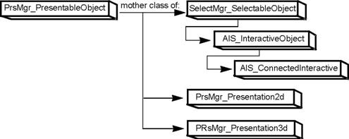
Interactive Objects are the entities, which are visualized and selected. You can use classes of standard interactive objects for which all necessary functions have already been programmed, or you can implement your own classes of interactive objects, by respecting a certain number of rules and conventions described below.

An Interactive Object is a "virtual" entity, which can be presented and selected. An Interactive Object can have a certain number of specific graphic attributes, such as visualization mode, color and material.
When an Interactive Object is visualized, the required graphic attributes are taken from its own Drawer if it has the required custom attributes or otherwise from the context drawer.
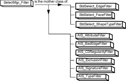
It can be necessary to filter the entities to be selected. Consequently there are Filter entities, which allow refining the dynamic detection context. Some of these filters can be used at the Neutral Point, others only in an open local context. It is possible to program custom filters and load them into the interactive context.
Entities which are visualized and selected in the AIS viewer are objects. They connect the underlying reference geometry of a model to its graphic representation in AIS. You can use the predefined OCCT classes of standard interactive objects, for which all necessary functions have already been programmed, or, if you are an advanced user, you can implement your own classes of interactive objects.
An interactive object can have as many presentations as its creator wants to give it.
3D presentations are managed by PresentationManager3D. As this is transparent in AIS, the user does not have to worry about it.
A presentation is identified by an index and by the reference to the Presentation Manager which it depends on.
By convention, the default mode of representation for the Interactive Object has index 0.
Calculation of different presentations of an interactive object is done by the Compute functions inheriting from PrsMgr_ PresentableObject::Compute functions. They are automatically called by PresentationManager at a visualization or an update request.
If you are creating your own type of interactive object, you must implement the Compute function in one of the following ways:
#### For hidden line removal (HLR) mode in 3D:
The view can have two states: the normal mode or the computed mode (Hidden Line Removal mode). When the latter is active, the view looks for all presentations displayed in the normal mode, which have been signalled as accepting HLR mode. An internal mechanism allows calling the interactive object's own Compute, that is projector function.
By convention, the Interactive Object accepts or rejects the representation of HLR mode. It is possible to make this declaration in one of two ways:
AIS_Shape class is an example of an interactive object that supports HLR representation. It supports two types of the HLR algorithm:
The type of the HLR algorithm is stored in AIS_Drawer of the shape. It is a value of the Prs3d_TypeOfHLR enumeration and can be set to:
The type of the HLR algorithm used for AIS_Shape can be changed by calling the AIS_Shape::SetTypeOfHLR() method.
The current HLR algorithm type can be obtained using AIS_Shape::TypeOfHLR() method is to be used.
These methods get the value from the drawer of AIS_Shape. If the HLR algorithm type in the AIS_Drawer is set to Prs3d_TOH_NotSet, the AIS_Drawer gets the value from the default drawer of AIS_InteractiveContext.
So it is possible to change the default HLR algorithm used by all newly displayed interactive objects. The value of the HLR algorithm type stored in the context drawer can be Prs3d_TOH_Algo or Prs3d_TOH_PolyAlgo. The polygonal algorithm is the default one.
There are four types of interactive objects in AIS:
Inside these categories, additional characterization is available by means of a signature (an index.) By default, the interactive object has a NONE type and a signature of 0 (equivalent to NONE.) If you want to give a particular type and signature to your interactive object, you must redefine two virtual functions:
Note that some signatures are already used by "standard" objects provided in AIS (see the List of Standard Interactive Object Classes.
The interactive context can have a default mode of representation for the set of interactive objects. This mode may not be accepted by a given class of objects.
Consequently, to get information about this class it is necessary to use virtual function AIS_InteractiveObject::AcceptDisplayMode.
The functions AIS_InteractiveContext::SetDisplayMode and AIS_InteractiveContext::UnsetDisplayMode allow setting a custom display mode for an objects, which can be different from that proposed by the interactive context.
At dynamic detection, the presentation echoed by the Interactive Context, is by default the presentation already on the screen.
The functions AIS_InteractiveObject::SetHilightMode and AIS_InteractiveObject::UnSetHilightMode allow specifying the display mode used for highlighting (so called highlight mode), which is valid independently from the active representation of the object. It makes no difference whether this choice is temporary or definitive.
Note that the same presentation (and consequently the same highlight mode) is used for highlighting detected objects and for highlighting selected objects, the latter being drawn with a special selection color (refer to the section related to Interactive Context services).
For example, you want to systematically highlight the wireframe presentation of a shape - non regarding if it is visualized in wireframe presentation or with shading. Thus, you set the highlight mode to 0 in the constructor of the interactive object. Do not forget to implement this representation mode in the Compute functions.
If you do not want an object to be affected by a FitAll view, you must declare it infinite; you can cancel its "infinite" status using AIS_InteractiveObject::SetInfiniteState and AIS_InteractiveObject::IsInfinite functions.
Let us take for example the class called IShape representing an interactive object :
An interactive object can have an indefinite number of selection modes, each representing a "decomposition" into sensitive primitives. Each primitive has an owner (SelectMgr_EntityOwner) which allows identifying the exact interactive object or shape which has been detected (see Selection chapter).
The set of sensitive primitives, which correspond to a given mode, is stocked in a selection (SelectMgr_Selection).
Each selection mode is identified by an index. By convention, the default selection mode that allows us to grasp the interactive object in its entirety is mode 0. However, it can be modified in the custom interactive objects using method SelectMgr_SelectableObject::setGlobalSelMode().
The calculation of selection primitives (or sensitive entities) is done by the intermediary of a virtual function, ComputeSelection. It should be implemented for each type of interactive object that is assumed to have different selection modes using the function AIS_ConnectedInteractive::ComputeSelection.
A detailed explanation of the mechanism and the manner of implementing this function has been given in Selection chapter.
There are some examples of selection mode calculation for the most widely used interactive object in OCCT – AIS_Shape (selection by vertex, by edges, etc). To create new classes of interactive objects with the same selection behavior as AIS_Shape – such as vertices and edges – you must redefine the virtual function AIS_InteractiveObject::AcceptShapeDecomposition.
You can change the default selection mode index of a custom interactive object using the following functions:
You also can temporarily change the priority of some interactive objects for selection of the global mode to facilitate their graphic detection using the following functions:
Graphic attributes manager, or AIS Drawer, stores graphic attributes for specific interactive objects and for interactive objects controlled by interactive context.
Initially, all drawer attributes are filled out with the predefined values which will define the default 3D object appearance.
When an interactive object is visualized, the required graphic attributes are first taken from its own drawer if one exists, or from the context drawer if no specific drawer for that type of object exists.
Keep in mind the following points concerning graphic attributes:

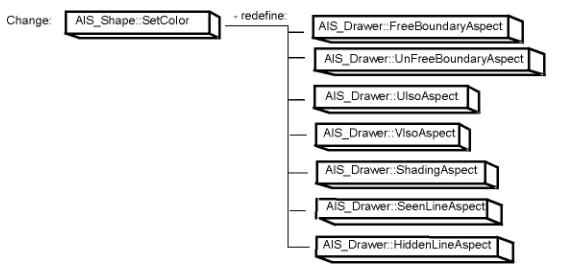
For other types of attribute, it is appropriate to change the Drawer of the object directly using:
It is important to know which functions may imply the recalculation of presentations of the object.
If the presentation mode of an interactive object is to be updated, a flag from PrsMgr_PresentableObject indicates this.
The mode can be updated using the functions Display and Redisplay in AIS_InteractiveContext.
When you use complementary services for interactive objects, pay special attention to the cases mentioned below.
The following functions allow temporarily "moving" the representation and selection of Interactive Objects in a view without recalculation.
Each Interactive Object has functions that allow attributing it an Owner in form of a Transient.
An interactive object can therefore be associated or not with an applicative entity, without affecting its behavior.
Due to the fact that the accuracy of three-dimensional graphics coordinates has a finite resolution the elements of topological objects can coincide producing the effect of "popping" some elements one over another.
To the problem when the elements of two or more Interactive Objects are coincident you can apply the polygon offset. It is a sort of graphics computational offset, or depth buffer offset, that allows you to arrange elements (by modifying their depth value) without changing their coordinates. The graphical elements that accept this kind of offsets are solid polygons or displayed as boundary lines and points. The polygons could be displayed as lines or points by setting the appropriate interior style.
The method AIS_InteractiveObject::SetPolygonOffsets (const Standard_Integer aMode, const Standard_Real aFactor, const Standard_Real aUnits) allows setting up the polygon offsets.
The parameter aMode can contain various combinations of Aspect_PolygonOffsetMode enumeration elements:
The combination of these elements defines the polygon display modes that will use the given offsets. You can switch off the polygon offsets by passing Aspect_POM_Off. Passing Aspect_POM_None allows changing the aFactor and aUnits values without changing the mode. If aMode is different from Aspect_POM_Off, the aFactor and aUnits arguments are used by the graphics renderer to calculate the depth offset value:
where m is the maximum depth slope for the currently displayed polygons, r is the minimum depth resolution (implementation-specific).
Negative offset values move polygons closer to the viewer while positive values shift polygons away.
Warning
This method has a side effect – it creates its own shading aspect if not yet created, so it is better to set up the object shading aspect first.
You can use the following functions to obtain the current settings for polygon offsets:
The same operation could be performed for the interactive object known by the AIS_InteractiveContext with the following methods:
The Interactive Context allows managing in a transparent way the graphic and selectable behavior of interactive objects in one or more viewers. Most functions which allow modifying the attributes of interactive objects, and which were presented in the preceding chapter, will be looked at again here.
There is one essential rule to follow: the modification of an interactive object, which is already known by the Context, must be done using Context functions. You can only directly call the functions available for an interactive object if it has not been loaded into an Interactive Context.
You can also write
Neutral Point and Local Context constitute the two operating modes or states of the Interactive Context, which is the central entity which pilots visualizations and selections.
The Neutral Point, which is the default mode, allows easily visualizing and selecting interactive objects, which have been loaded into the context. Opening Local contexts allows preparing and using a temporary selection environment without disturbing the neutral point.
A set of functions allows choosing the interactive objects which you want to act on, the selection modes which you want to activate, and the temporary visualizations which you will execute. When the operation is finished, you close the current local context and return to the state in which you were before opening it (neutral point or previous local context).
The Interactive Context is composed of many functions, which can be conveniently grouped according to the theme:
Some functions can only be used in open Local Context; others in closed local context; others do not have the same behavior in one state as in the other.
The Interactive Context is made up of a Principal Viewer and, optionally, a trash bin or Collector Viewer.
An interactive object can have a certain number of specific graphic attributes, such as visualization mode, color, and material. Correspondingly, the interactive context has a set of graphic attributes, the Drawer, which is valid by default for the objects it controls.
When an interactive object is visualized, the required graphic attributes are first taken from the object's own Drawer if one exists, or from the context drawer for the others.
The following adjustable settings allow personalizing the behavior of presentations and selections:
All of these settings can be modified by functions proper to the Context.
When you change a graphic attribute pertaining to the Context (visualization mode, for example), all interactive objects, which do not have the corresponding appropriate attribute, are updated.
Let us examine the case of two interactive objects: obj1 and obj2:
PresentationManager3D and Selector3D, which manage the presentation and selection of present interactive objects, are associated to the main Viewer. The same is true of the optional Collector.
The interactive object, which is used the most by applications, is AIS_Shape. Consequently, standard functions are available which allow you to easily prepare selection operations on the constituent elements of shapes (selection of vertices, edges, faces etc) in an open local context. The selection modes specific to "Shape" type objects are called Standard Activation Mode. These modes are only taken into account in open local context and only act on interactive objects which have redefined the virtual function AcceptShapeDecomposition() so that it returns TRUE.
Warning
The specific modes of selection only concern the interactive objects, which are present in the Main Viewer. In the Collector, you can only locate interactive objects, which answer positively to the positioned filters when a local context is open, however, they are never decomposed in standard mode.
The local context can be opened using method AIS_InteractiveContext::OpenLocalContext. The following options are available:
This function returns the index of the created local context. It should be kept and used when the context is closed.
To load objects visualized at Neutral Point into a local context or remove them from it use methods
Closing Local Contexts is done by:
Warning When the index is not specified in the first function, the current Context is closed. This option can be dangerous, as other Interactive Functions can open local contexts without necessarily warning the user. For greater security, you have to close the context with the index given on opening.
To get the index of the current context, use function AIS_InteractiveContext::IndexOfCurrentLocal. It allows closing all open local contexts at one go. In this case, you find yourself directly at Neutral Point.
When you close a local context, all temporary interactive objects are deleted, all selection modes concerning the context are canceled, and all content filters are emptied.
You must distinguish between the Neutral Point and the Open Local Context states. Although the majority of visualization functions can be used in both situations, their behavior is different.
Neutral Point should be used to visualize the interactive objects, which represent and select an applicative entity. Visualization and Erasing orders are straightforward:
Bear in mind the following points:
In open local context, the Display functions presented above can be as well.
WARNING
The function AIS_InteractiveObject::Display automatically activates the object's default selection mode. When you only want to visualize an Interactive Object in open Context, you must call the function AIS_InteractiveContext::Display.
You can activate or deactivate specific selection modes in the local open context in several different ways: Use the Display functions with the appropriate modes.
This activates the corresponding selection mode for all objects in Local Context, which accept decomposition into sub-shapes. Every new Object which has been loaded into the interactive context and which meets the decomposition criteria is automatically activated according to these modes.
WARNING
If you have opened a local context by loading an object with the default options (AllowShapeDecomposition = Standard_True), all objects of the "Shape" type are also activated with the same modes. You can change the state of these "Standard" objects by using SetShapeDecomposition(Status).
Load an interactive object by the function AIS_InteractiveContext::Load.
This function allows loading an Interactive Object whether it is visualized or not with a given selection mode, and/or with the necessary decomposition option. If AllowDecomp=TRUE and obviously, if the interactive object is of the "Shape" type, these "standard" selection modes will be automatically activated as a function of the modes present in the Local Context.
Use AIS_InteractiveContext::Activate and AIS_InteractiveContext::Deactivate to directly activate/deactivate selection modes on an object.
To define an environment of dynamic detection, you can use standard filter classes or create your own. A filter questions the owner of the sensitive primitive in local context to determine if it has the desired qualities. If it answers positively, it is kept. If not, it is rejected.
The root class of objects is SelectMgr_Filter. The principle behind it is straightforward: a filter tests to see whether the owners (SelectMgr_EntityOwner) detected in mouse position by the Local context selector answer OK. If so, it is kept, otherwise it is rejected.
You can create a custom class of filter objects by implementing the deferred function IsOk():
In SelectMgr, there are also Composition filters (AND Filters, OR Filters), which allow combining several filters. In InteractiveContext , all filters that you add are stocked in an OR filter (which answers OK if at least one filter answers OK).
There are Standard filters, which have already been implemented in several packages:
As there are specific behaviors on shapes, each new Filter class must, if necessary, redefine AIS_LocalContext::ActsOn function, which informs the Local Context if it acts on specific types of sub-shapes. By default, this function answers FALSE.
WARNING
Only type filters are activated in Neutral Point to make it possible to identify a specific type of visualized object. For filters to come into play, one or more object selection modes must be activated.
There are several functions to manipulate filters:
Dynamic detection and selection are put into effect in a straightforward way. There are only a few conventions and functions to be familiar with. The functions are the same in neutral point and in open local context:
Highlighting of detected and selected entities is automatically managed by the Interactive Context, whether you are in neutral point or Local Context. The Highlight colors are those dealt with above. You can nonetheless disconnect this automatic mode if you want to manage this part yourself :
If there is no open local context, the objects selected are called current objects. If there is a local context, they are called selected objects. Iterators allow entities to be recovered in either case. A set of functions allows manipulating the objects, which have been placed in these different lists.
WARNING
When a Local Context is open, you can select entities other than interactive objects (vertices, edges etc.) from decompositions in standard modes, or from activation in specific modes on specific interactive objects. Only interactive objects are stocked in the list of selected objects.
You can question the Interactive context by moving the mouse. The following functions can be used:
After using the Select and ShiftSelect functions in Neutral Point, you can explore the list of selections, referred to as current objects in this context. The following functions can be used:
In the Local Context, you can explore the list of selected objects available. The following functions can be used:
You have to ask whether you have selected a shape or an interactive object before you can recover the entity in the Local Context or in the iteration loop. If you have selected a Shape from TopoDS on decomposition in standard mode, the Interactive() function returns the interactive object, which provided the selected shape. Other functions allow you to manipulate the content of Selected or Current Objects:
You can highlight and remove highlighting from a current object, and empty the list of current objects using the following functions:
When you are in an open Local Context, you may need to keep "temporary" interactive objects. This is possible using the following functions:
You can also want to use function AIS_InteractiveContext::ClearLocalContext to modify in a general way the state of the local context before continuing a selection (emptying objects, removing filters, standard activation modes).
The possibilities of use for local contexts are numerous depending on the type of operation that you want to perform:
When you want to work on one type of entity, you should open a local context with the option UseDisplayedObjects set to FALSE. Some functions which allow you to recover the visualized interactive objects, which have a given Type, and Signature from the "Neutral Point" are:
At this stage, you only have to load the functions Load, Activate, and so on.
When you open a Local Context with default options, you must keep the following points in mind:
The stages could be the following:
It is useful to create an interactive editor, to which you pass the Interactive Context. This allow setting up different contexts of selection/presentation according to the operation, which you want to perform.
Let us assume that you have visualized several types of interactive objects: AIS_Points, AIS_Axes, AIS_Trihedrons, and AIS_Shapes.
For your applicative function, you need an axis to create a revolved object. You could obtain this axis by identifying:
Interactive Objects are selectable and viewable objects connecting graphic representation and the underlying reference geometry.
They are divided into four types:
Inside these categories, there is a possibility of additional characterization by means of a signature. The signature provides an index to the further characterization. By default, the Interactive Object has a None type and a signature of 0 (equivalent to None). If you want to give a particular type and signature to your interactive object, you must redefine the two virtual methods: Type and Signature.
The Datum groups together the construction elements such as lines, circles, points, trihedrons, plane trihedrons, planes and axes.
AIS_Point, AIS_Axis, AIS_Line, AIS_Circle, AIS_Plane and AIS_Trihedron have four selection modes:
when you activate one of modes: 1 2 3 4, you pick AIS objects of type:
AIS_PlaneTrihedron offers three selection modes:
For the presentation of planes and trihedra, the default unit of length is millimeter, and the default value for the representation of axes is 100. If you modify these dimensions, you must temporarily recover the object Drawer. From it, take the Aspects in which the values for length are stored (PlaneAspect for the plane, FirstAxisAspect for trihedra), and change these values inside these Aspects. Finally, recalculate the presentation.
The Object type includes topological shapes, and connections between shapes.
AIS_Shape has three visualization modes :
And at maximum seven selection modes, depending on the shape complexity:
The class AIS_ColoredShape allows using custom colors and line widths for TopoDS_Shape objects and their sub-shapes.
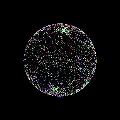
The presentation class AIS_PointCloud can be used for efficient drawing of large arbitrary sets of colored points. It uses Graphic3d_ArrayOfPoints to pass point data into OpenGl graphic driver to draw a set points as an array of "point sprites". The point data is packed into vertex buffer object for performance.
Example:
The draw command vpointcloud builds a cloud of points from shape triangulation. This command can also draw a sphere surface or a volume with a large amount of points (more than one million).
The Relation is made up of constraints on one or more interactive shapes and the corresponding reference geometry. For example, you might want to constrain two edges in a parallel relation. This constraint is considered as an object in its own right, and is shown as a sensitive primitive. This takes the graphic form of a perpendicular arrow marked with the || symbol and lying between the two edges.
The following relations are provided by AIS:
The list of relations is not exhaustive.
MeshVS_Mesh is an Interactive Object that represents meshes. This object differs from the AIS_Shape as its geometrical data is supported by the data source MeshVS_DataSource that describes nodes and elements of the object. As a result, you can provide your own data source.
However, the DataSource does not provide any information on attributes, for example nodal colors, but you can apply them in a special way – by choosing the appropriate presentation builder.
The presentations of MeshVS_Mesh are built with the presentation builders MeshVS_PrsBuilder. You can choose between the builders to represent the object in a different way. Moreover, you can redefine the base builder class and provide your own presentation builder.
You can add/remove builders using the following methods:
There is a set of reserved display and highlighting mode flags for MeshVS_Mesh. Mode value is a number of bits that allows selecting additional display parameters and combining the following mode flags, which allow displaying mesh in wireframe, shading and shrink modes:
It is also possible to display deformed mesh in wireframe, shading or shrink modes usung :
The following methods represent different kinds of data :
The following methods provide selection and highlighting :
MeshVS_DMF_User is a user-defined mode.
These values will be used by the presentation builder. There is also a set of selection modes flags that can be grouped in a combination of bits:
Such an object, for example, can be used for displaying the object and stored in the STL file format:
MeshVS_NodalColorPrsBuilder allows representing a mesh with a color scaled texture mapped on it. To do this you should define a color map for the color scale, pass this map to the presentation builder, and define an appropriate value in the range of 0.0 - 1.0 for every node.
The following example demonstrates how you can do this (check if the view has been set up to display textures):
The dynamic selection represents the topological shape, which you want to select, by decomposition of sensitive primitives – the sub-parts of the shape that will be detected and highlighted. The sets of these primitives are handled by the powerful three-level BVH tree selection algorithm.
For more details on the algorithm and examples of usage, please, refer to Selection chapter.
The Graphic3d package is used to create 3D graphic objects in a 3D viewer. These objects called structures are made up of groups of primitives and attributes, such as polylines, planar polygons with or without holes, text and markers, and attributes, such as color, transparency, reflection, line type, line width, and text font. A group is the smallest editable element of a structure. A transformation can be applied to a structure. Structures can be connected to form a tree of structures, composed by transformations. Structures are globally manipulated by the viewer.
Graphic structures can be:
There are classes for:
The root is the top of a structure hierarchy or structure network. The attributes of a parent structure are passed to its descendants. The attributes of the descendant structures do not affect the parent. Recursive structure networks are not supported.
Primitive arrays are a more efficient approach to describe and display the primitives from the aspects of memory usage and graphical performance. The key feature of the primitive arrays is that the primitive data is not duplicated. For example, two polygons could share the same vertices, so it is more efficient to keep the vertices in a single array and specify the polygon vertices with indices of this array. In addition to such kind of memory savings, the OpenGl graphics driver provides the Vertex Buffer Objects (VBO). VBO is a sort of video memory storage that can be allocated to hold the primitive arrays, thus making the display operations more efficient and releasing the RAM memory.
The Vertex Buffer Objects are enabled by default, but VBOs availability depends on the implementation of OpenGl. If the VBOs are unavailable or there is not enough video memory to store the primitive arrays, the RAM memory will be used to store the arrays.
The Vertex Buffer Objects can be disabled at the application level. You can use the method Graphic3d_GraphicDriver::EnableVBO (const Standard_Boolean status) to enable/disable VBOs:
The following example shows how to disable the VBO support:
Note that the use of Vertex Buffer Objects requires the application level primitive data provided by the Graphic3d_ArrayOfPrimitives to be transferred to the video memory. TKOpenGl transfers the data and releases the Graphic3d_ArrayOfPrimitives internal pointers to the primitive data. Thus it might be necessary to pay attention to such kind of behaviour, as the pointers could be modified (nullified) by the TKOpenGl.
The different types of primitives could be presented with the following primitive arrays:
The Graphic3d_ArrayOfPrimitives is a base class for these primitive arrays.
Method Graphic3d_ArrayOfPrimitives::AddVertex allows adding There is a set of similar methods to add vertices to the primitive array.
These methods take vertex coordinates as an argument and allow you to define the color, the normal and the texture coordinates assigned to the vertex. The return value is the actual number of vertices in the array.
You can also modify the values assigned to the vertex or query these values by the vertex index:
The following example shows how to define an array of points:
If the primitives share the same vertices (polygons, triangles, etc.) then you can define them as indices of the vertices array.
The method Graphic3d_ArrayOfPrimitives::AddEdge allows defining the primitives by indices. This method adds an "edge" in the range [1, VertexNumber() ] in the array.
It is also possible to query the vertex defined by an edge using method Graphic3d_ArrayOfPrimitives::Edge
The following example shows how to define an array of triangles:
If the primitive array presents primitives built from sequential sets of vertices, for example polygons, then you can specify the bounds, or the number of vertices for each primitive. You can use the method Graphic3d_ArrayOfPrimitives::AddBound to define the bounds and the color for each bound. This method returns the actual number of bounds.
It is also possible to set the color and query the number of edges in the bound and bound color.
The following example shows how to define an array of polygons:
There are also several helper methods. You can get the type of the primitive array:
and check if the primitive array provides normals, vertex colors and vertex texels (texture coordinates):
or get the number of vertices, edges and bounds:
The OpenGl graphics driver uses advanced text rendering powered by FTGL library. This library provides vector text rendering, as a result the text can be rotated and zoomed without quality loss. Graphic3d text primitives have the following features:
The text attributes for the group could be defined with the Graphic3d_AspectText3d attributes group. To add any text to the graphic structure you can use the following methods:
AText parameter is the text string, APoint is the three-dimensional position of the text, AHeight is the text height, AAngle is the orientation of the text (at the moment, this parameter has no effect, but you can specify the text orientation through the Graphic3d_AspectText3d attributes).
ATp parameter defines the text path, AHta is the horizontal alignment of the text, AVta is the vertical alignment of the text.
You can pass Standard_False as EvalMinMax if you do not want the graphic3d structure boundaries to be affected by the text position.
Note that the text orientation angle can be defined by Graphic3d_AspectText3d attributes.
See the example:
A Graphic3d_MaterialAspect is defined by:
The following items are required to determine the three colors of reflection:
A texture is defined by a name. Three types of texture are available:
OCCT visualization core supports GLSL shaders. Currently OCCT supports only vertex and fragment GLSL shader. Shaders can be assigned to a generic presentation by its drawer attributes (Graphic3d aspects). To enable custom shader for a specific AISShape in your application, the following API functions are used:
The Aspect package provides classes for the graphic elements in the viewer:
The V3d package provides the resources to define a 3D viewer and the views attached to this viewer (orthographic, perspective). This package provides the commands to manipulate the graphic scene of any 3D object visualized in a view on screen.
A set of high-level commands allows the separate manipulation of parameters and the result of a projection (Rotations, Zoom, Panning, etc.) as well as the visualization attributes (Mode, Lighting, Clipping, Depth-cueing, etc.) in any particular view.
The V3d package is basically a set of tools directed by commands from the viewer front-end. This tool set contains methods for creating and editing classes of the viewer such as:
This sample TEST program for the V3d Package uses primary packages Xw and Graphic3d and secondary packages Visual3d, Aspect, Quantity, Phigs and math.
As an alternative to manual setting of perspective parameters the V3d_View::ZfitAll() and V3d_View::FitAll() functions can be used:
View projection and orientation in OCCT v3d view are driven by camera. The camera calculates and supplies projection and view orientation matrices for rendering by OpenGL. The allows to the user to control all projection parameters. The camera is defined by the following properties:
Most common view manipulations (panning, zooming, rotation) are implemented as convenience methods of V3d_View class, however Graphic3d_Camera class can also be used directly by application developers:
Example:
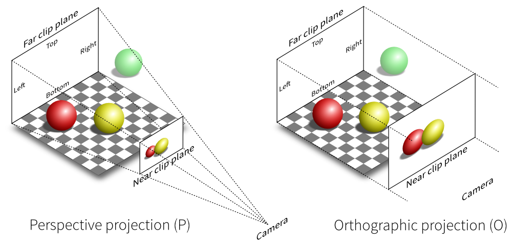
The following code configures the camera for orthographic rendering:
Field of view (FOVy) – defines the field of camera view by y axis in degrees (45� is default).
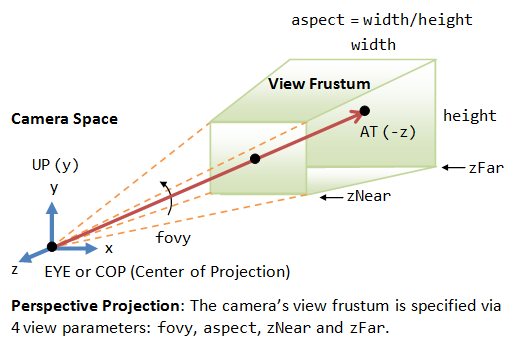
The following code configures the camera for perspective rendering:
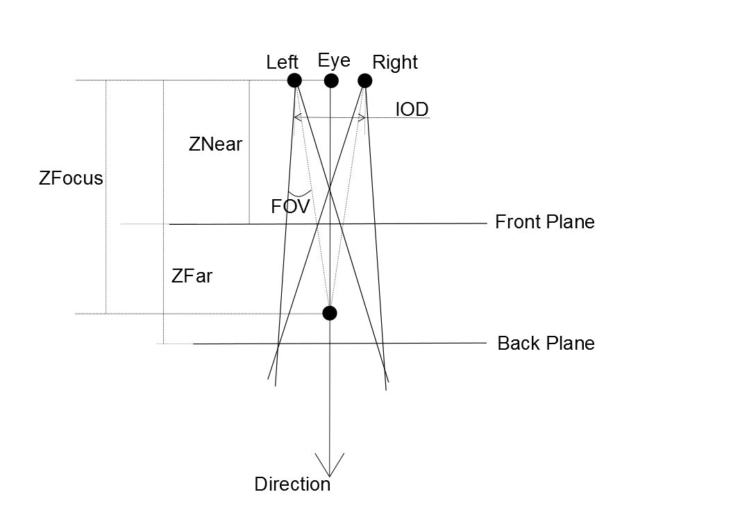
IOD – defines the intraocular distance (in world space units).
There are two types of IOD:
Field of view (FOV) – defines the field of camera view by y axis in degrees (45� is default).
ZFocus – defines the distance to the point of stereographic focus.
To enable stereo projection, your workstation should meet the following requirements:
In stereographic projection mode the camera prepares two projection matrices to display different stereo-pictures for the left and for the right eye. In a non-stereo camera this effect is not visible because only the same projection is used for both eyes.
To enable quad buffering support you should provide the following settings to the graphic driver opengl_caps:
The following code configures the camera for stereographic rendering:
The algorithm of frustum culling on CPU-side is activated by default for 3D viewer. This algorithm allows skipping the presentation outside camera at the rendering stage, providing better performance. The following features support this method:
In addition to interactive 3d graphics displayed in the view you can display underlying and overlying graphics: text, color scales and drawings.
All V3d view graphical objects in the overlay are managed by the default layer manager (V3d_LayerMgr). The V3d view has a basic layer manager capable of displaying the color scale, but you can redefine this class to provide your own overlay and underlay graphics.
The method V3d_View::SetLayerMgr(const Handle (V3d_LayerMgr)& aMgr) allows assigning a custom layer manager to the V3d view.
There are three virtual methods to prepare graphics in the manager for further drawing: setting up layer dimensions and drawing static graphics. These methods can be redefined:
The layer manager controls layers (Visual3d_Layer) and layer items (Visual3d_LayerItem). Both the overlay and underlay layers can be created by the layer manager.
The layer entity is presented by the Visual3d_Layer class. This entity provides drawing services in the layer, for example:
The following example demonstrates how to draw overlay graphics by the V3d_LayerMgr:
The layer contains layer items that will be displayed on view redraw. Such items are Visual3d_LayerItem entities. To manipulate Visual3d_LayerItem entities assigned to the layer's internal list you can use the following methods:
The layer's items are rendered when the method void Visual3d_Layer::RenderLayerItems() is called by the graphical driver.
The Visual3d_LayerItem has virtual methods that are used to render the item:
The item presentation can be computed before drawing by the ComputeLayerPrs method to save time on redraw. It also has an additional flag that is used to tell that the presentation should be recomputed:
An example of Visual3d_LayerItem is V3d_ColorScaleLayerItem that represents the color scale entity as the layer's item. The V3d_ColorScaleLayerItem sends render requests to the color scale entity represented by it. As this entity (V3d_ColorScale) is assigned to the V3d_LayerMgr it uses its overlay layer's services for drawing:
There are three types of background styles available for V3d_view: solid color, gradient color and image.
To set solid color for the background you can use the following methods:
This method allows you to specify the background color in RGB (red, green, blue) or HLS (hue, lightness, saturation) color spaces, so the appropriate values of the Type parameter are Quantity_TOC_RGB and Quantity_TOC_HLS.
Note that the color value parameters V1,V2,V3 should be in the range between 0.0-1.0.
The gradient background style could be set up with the following methods:
The Color1 and Color2 parameters define the boundary colors of interpolation, the FillStyle parameter defines the direction of interpolation. You can pass Standard_True as the last parameter to update the view.
The fill style can be also set with the method void V3d_View::SetBgGradientStyle(const Aspect_GradientFillMethod AMethod, const Standard_Boolean update).
To get the current background color you can use the following methods:
To set the image as a background and change the background image style you can use the following methods:
The FileName parameter defines the image file name and the path to it, the FillStyle parameter defines the method of filling the background with the image. The methods are:
The 3D scene displayed in the view can be dumped in high resolution into an image file. The high resolution (8192x8192 on some implementations) is achieved using the Frame Buffer Objects (FBO) provided by the graphic driver. Frame Buffer Objects enable off-screen rendering into a virtual view to produce images in the background mode (without displaying any graphics on the screen).
The V3d_View has the following methods for dumping the 3D scene:
Dumps the scene into an image file with the view dimensions.
Makes the dimensions of the output image compatible to a certain format of printing paper passed by theFormat argument.
These methods dump the 3D scene into an image file passed by its name and path as theFile.
The raster image data handling algorithm is based on the Image_PixMap class. The supported extensions are ".png", ".bmp", ".png", ".png".
The value passed as theBufferType argument defines the type of the buffer for an output image (RGB, RGBA, floating-point, RGBF, RGBAF). Both methods return Standard_True if the scene has been successfully dumped.
There is also class Image_AlienPixMap providing import / export from / to external image files in formats supported by FreeImage library.
Note that dumping the image for a paper format with large dimensions is a memory consuming operation, it might be necessary to take care of preparing enough free memory to perform this operation.
Dumps the displayed 3d scene into a pixmap with a width and height passed as theWidth and theHeight arguments.
The value passed as theBufferType argument defines the type of the buffer for a pixmap (RGB, RGBA, floating-point, RGBF, RGBAF). The last parameter allows centering the 3D scene on dumping.
All these methods assume that you have created a view and displayed a 3d scene in it. However, the window used for such a view could be virtual, so you can dump the 3d scene in the background mode without displaying it on the screen. To use such an opportunity you can perform the following steps:
The following example demonstrates this procedure for WNT_Window :
The contents of a view can be printed out. Moreover, the OpenGl graphic driver used by the v3d view supports printing in high resolution. The print method uses the OpenGl frame buffer (Frame Buffer Object) for rendering the view contents and advanced print algorithms that allow printing in, theoretically, any resolution.
The method void V3d_View::Print(const Aspect_Handle hPrnDC, const Standard_Boolean showDialog, const Standard_Boolean showBackground, const Standard_CString filename, const Aspect_PrintAlgo printAlgorithm) prints the view contents:
hPrnDC is the printer device handle. You can pass your own printer handle or NULL to select the printer by the default dialog. In that case you can use the default dialog or pass Standard_False as the showDialog argument to select the default printer automatically.
You can define the filename for the printer driver if you want to print out the result into a file. If you do not want to print the background, you can pass Standard_False as the showBackground argument. The printAlgorithm argument allows choosing between two print algorithms that define how the 3d scene is mapped to the print area when the maximum dimensions of the frame buffer are smaller than the dimensions of the print area by choosing Aspect_PA_STRETCH or Aspect_PA_TILE
The first value defines the stretch algorithm: the scene is drawn with the maximum possible frame buffer dimensions and then is stretched to the whole printing area. The second value defines TileSplit algorithm: covering the whole printing area by rendering multiple parts of the viewer.
Note that at the moment the printing is implemented only for Windows.
The 3D content of a view can be exported to the vector image file format. The vector image export is powered by the GL2PS library. You can export 3D scenes into a file format supported by the GL2PS library: PostScript (PS), Encapsulated PostScript (EPS), Portable Document Format (PDF), Scalable Vector Graphics (SVG), LaTeX file format and Portable LaTeX Graphics (PGF).
The method void Visual3d_View::Export (const Standard_CString FileName, const Graphic3d_ExportFormat Format, const Graphic3d_SortType aSortType, const Standard_Real Precision, const Standard_Address ProgressBarFunc, const Standard_Address ProgressObject) of Visual3d_View class allows exporting a 3D scene:
The FileName defines the output image file name and the Format argument defines the output file format:
The aSortType parameter defines GL2PS sorting algorithm for the primitives. The Precision, ProgressBarFunc and ProgressObject parameters are implemented for future uses and at the moment have no effect.
The Export method supports only basic 3d graphics and has several limitations:
OCCT visualization provides rendering by real-time ray tracing technique. It is allowed to switch easily between usual rasterization and ray tracing rendering modes. The core of OCCT ray tracing is written using GLSL shaders. The ray tracing has a wide list of features:
The ray tracing algorithm is recursive (Whitted's algorithm). It uses BVH effective optimization structure. The structure prepares optimized data for a scene geometry for further displaying it in real-time. The time-consuming re-computation of the BVH is not necessary for view operations, selections, animation and even editing of the scene by transforming location of the objects. It is only necessary when the list of displayed objects or their geometry changes. To make the BVH reusable it has been added into an individual reusable OCCT package TKMath/BVH.
There are several ray-tracing options that user can switch on/off:
Example:
Structure display priorities control the order, in which structures are drawn. When you display a structure you specify its priority. The lower is the value, the lower is the display priority. When the display is regenerated, the structures with the lowest priority are drawn first. The structures with the same display priority are drawn in the same order as they have been displayed. OCCT supports eleven structure display priorities.
OCCT features depth-arranging functionality called z-layer. A graphical presentation can be put into a z-layer. In general, this function can be used for implementing "bring to front" functionality in a graphical application.
Example:
For each z-layer, it is allowed to:
The corresponding method SetZLayerOption (...) is available in Graphic3d_GraphicDriver interface. You can get the options using getter from Visual3d_ViewManager and V3d_Viewer. It returns Graphic3d_ZLayerSettings cached in Visual3d_ViewManager for a given LayerId.
Example:
The ability to define custom clipping planes could be very useful for some tasks. OCCT provides such an opportunity.
The Graphic3d_ClipPlane class provides the services for clipping planes: it holds the plane equation coefficients and provides its graphical representation. To set and get plane equation coefficients you can use the following methods:
The clipping planes can be activated with the following method:
The number of clipping planes is limited. You can check the limit value via method Graphic3d_GraphicDriver::InquirePlaneLimit();
Let us see for example how to create a new clipping plane with custom parameters and add it to a view or to an object:
Back face culling reduces the rendered number of triangles (which improves the performance) and eliminates artifacts at shape boundaries. However, this option can be used only for solid objects, where the interior is actually invisible from any point of view. Automatic back-face culling mechanism is turned on by default, which is controlled by V3d_View::SetBackFacingModel().
The following features are applied in StdPrs_ToolShadedShape::IsClosed(), which is used for definition of back face culling in ShadingAspect:
Back face culling is turned off at TKOpenGl level in the following cases:
To create 3D graphic objects and display them in the screen, follow the procedure below:
Create colors.
Create line attributes.
Create marker attributes.
Create facet attributes.
Create text attributes.
It is assumed that a valid Windows window may already be accessed via the method GetSafeHwnd().
You are now able to display interactive objects such as an AIS_Shape.
Follow the procedure below to compute the presentable object:
Note that there are two compute methods: one for a standard representation, and the other for a degenerated representation, i.e. in hidden line removal and wireframe modes.
Let us look at the example of compute methods
Get the group used in Prs3d_Presentation.
Update the group attributes.
Create two triangles in aGroup.
The methods BeginPrimitives() and EndPrimitives() are used when creating a set of various primitives in the same group. Use the polyline function to create a boundary box for the thePrs structure in group aGroup.
Create text and markers in group aGroup.
MeshVS (Mesh Visualization Service) component extends 3D visualization capabilities of Open CASCADE Technology. It provides flexible means of displaying meshes along with associated pre- and post-processor data.
From a developer's point of view, it is easy to integrate the MeshVS component into any mesh-related application with the following guidelines:
Visual attributes of the MeshVS_Mesh object (such as shading color, shrink coefficient and so on) are controlled through MeshVS_Drawer object. It maintains a map "Attribute ID --> attribute value" and can be easily extended with any number of custom attributes.
In all other respects, MeshVS_Mesh is very similar to any other class derived from AIS_InteractiveObject and it should be used accordingly (refer to the description of AIS package in the documentation).
 1.8.10